24. Text: Interpreting Interactions

Interaction Terms

In the previous video, you were introduced to how you might interpret interactions, and how you might observe the need for an interaction in your model.

Mathematically, an interaction is created by multiplying two variables by one another and adding this term to our linear regression model.

The example from the previous video used area (x_1) and the neighborhood (x_2) of a home (either A or B) to predict the home price (y). At the top of the screen in the video, you might have noticed the equation for a linear model using these variables as:

\hat{y} = b_0 + b_1x_1 + b_2x_2

This example does not involve an interaction term, and this model is appropriate if the relationship of the variables looks like that in the plot below.

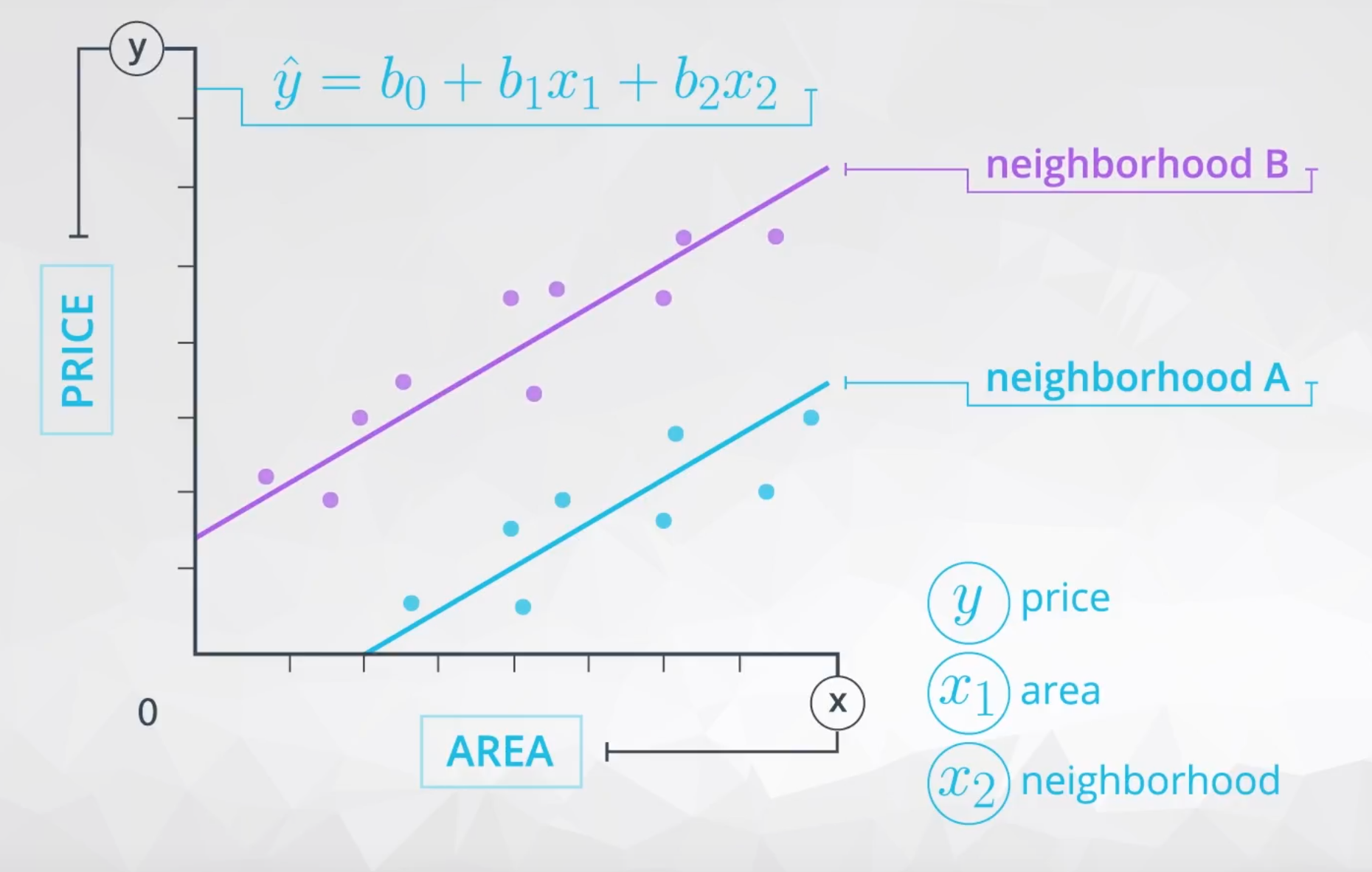
where b_1 is the way we estimate the relationship between area and price, which in this model we believe to be the same regardless of the neighborhood.

Then b_2 is the difference in price depending on which neighborhood you are in, which is the vertical distance between the two lines here:

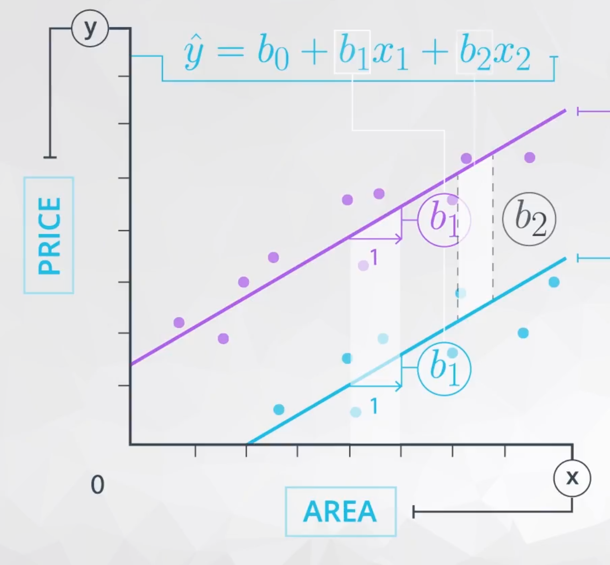
Notice here that:

• The way that area is related to price is the same regardless of neighborhood.

AND

• The difference in price for the different neighborhoods is the same regardless of the area.

When these statements are true, we do not need an interaction term in our model. However, we need an interaction when the way that area is related to price is different depending on the neighborhood.

Mathematically, when the way area relates to price depends on the neighborhood, this suggests we should add an interaction. By adding the interaction, we allow the slopes of the line for each neighborhood to be different, as shown in the plot below. Here we have added the interaction, and you can see this allows for a difference in these two slopes.

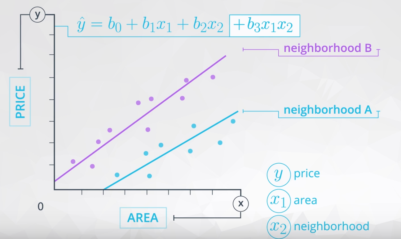
These lines might even cross or grow apart quickly. Either of these would suggest an interaction is present between area and neighborhood in the way they related to the price.